Crashworthiness of Carbon Fiber Composites
Instructions for Test Data Analysis
Instructions are copied from the project High Strain Rate Characterization of Magnesium Alloys. The process for analyzing data from the composite crashworthiness tests on this web site is essentially the same, and can be performed by following the steps below.
Step 1: Select Tests for Viewing
To analyze the data from the tests, first select the tests by checking check-boxes on the right. You can select multiple tests for comparison. Tests are grouped by material types and grades.The tests for other materials will be conducted as the materials become available.
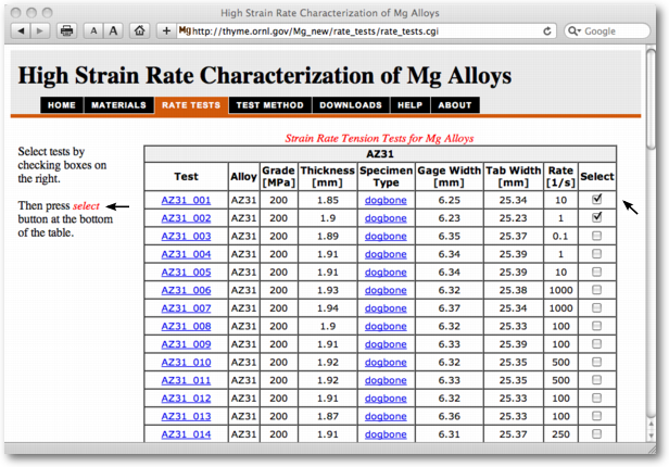
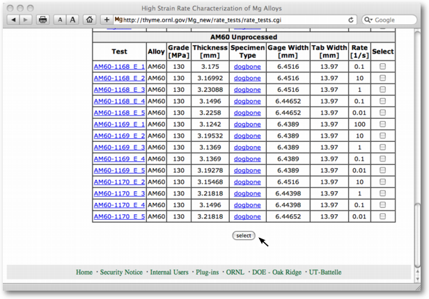
Once tests of interests are marked, scroll down to the bottom of the page and press select button. A quick way to scroll to the bottom of the page is to click on the hyperlink in the left column.
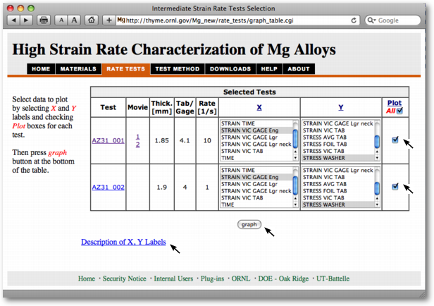
Step 2: Select Data from Tests to Analyze
Each test contain data from multiple sensors. The definition of test labels can be found by clicking on the link Description of X, Y Labels. Data sets from different tests is selected in X and Y columns of the test table. Only one X item in each test can be selected. Multiple Y items for each test may be selected using standard options in your browser.
The X data has to be of the same type, i.e. selected X labels for all tests to be analyzed have to start with same string, TIME or STRAIN. The Y data also have to be of the same type, i.e. selected Y labels for all tests to be displayed have to start with STRAIN or STRESS.
Test data is included into the graph by checking Plot check-box for the test. Multiple tests may be selected. Generate the graph in a new window by clicking graph button.
Strain derived from LVDT and TIME include the displacement of the overall load train, so that the material will appear more flexible than it is. This excess deformation can be determined and eventually subtracted by examining material deformation in the low strain region (yield region) using direct strain measurement methods. To do so, select X data set as STRAIN FOIL GAGE (electrical resistance strain gage bonded to the gage section of the specimen), or STRAIN VIC GAGE (strain measured by the digital image correlation in the specimen's gage section). The electrical resistance strain gages often debond at larger strains, especially for higher strain rates. In those cases, the data from STRAIN LVDT and/or STRAIN TIME can be appended to the low strain region data, although we need to account for the additional deformation that comes from the entire load train. A simple approach is to:
- select a Y value common to the X data sets for STRAIN (FOIL or VIC) GAGE (low strain region) and STRAIN (LVDT or TIME) (high strain region), and
- use the low strain region X point for the common Y value as the starting value for the large strain region data from STRAIN (LVDT or TIME).
Measurements from different sensors have different validity regions:
- Stress derived from LOADCELL data is the most reliable source for the stress data in the lowest strain rate range [0.01, 0.1] /sec.
- Load WASHER data is the most reliable source for stress data in the strain rate region [1, 10] /sec.
- Due to signal delay and inertia effect in the above two sensors, the stress measurements in the strain rate regime [50,1000] /sec are based on contact and optical measurement of strains at different locations of the specimen. The stress in the specimen is calculated based on simple elastic relation between stress and strain in elastically deformed tab region. Load WASHER data provides guide for the expected values, but its signals exhibits large oscillations.
Step 3: Display and Download Data
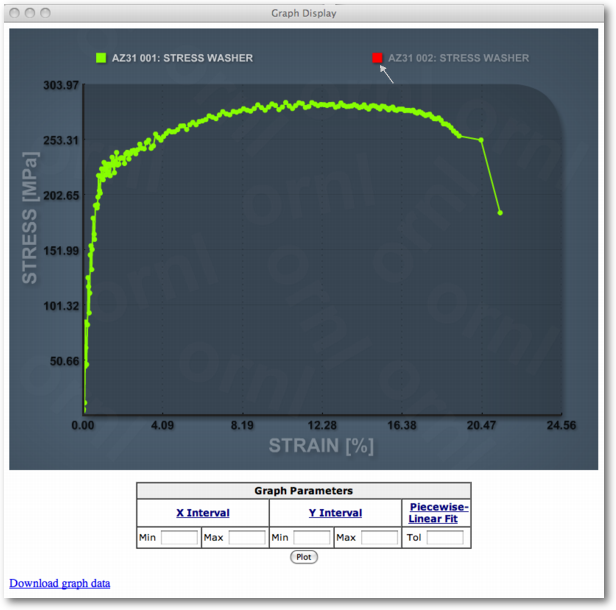
If selected data from the tests is compatible, a new window with the resulting graph will open.
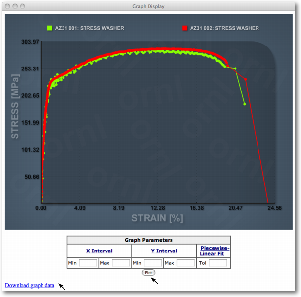
The data region of interest can be modified by specifying X Interval and Y Interval and pressing the Plot button. Data can be downloaded by clicking on Download graph data link. Print or save the graph image by mouse right-click inside the graph.
To reset a specific limit of the display region, just delete the content of the respective Min and/or Max boxes.
Data curves can be toggled in the graph display by clicking on the curve labels in the legend.
Step 4: Additional Data Processing and Download
You can also generate optimal piecewise linear interpolation for all the test data curves in the displayed graph by specifying tolerance parameter Tol and clicking on Plot button. The tolerance parameter is specified as a fraction of the total Y data range for the data, e.g. tolerance parameter value of 0.02 corresponds to 2% of the Y test data range.
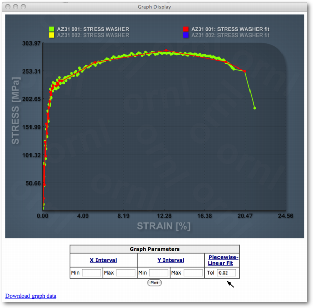
Interpolated curves are included in Download graph data link. These curves can be used for material models such as Piecewise Linear Plasticity Model in LS-DYNA. Note that the data first has to be converted into true stress - true strain form.